Halloween Lasts One Night. The Business Behind It Runs All Year.
A data science case study on the business of Halloween. Walmart and wholesale data from Hugging Face show when stock is bought, when shoppers buy, and how much a store should order when it can't know, with the full notebook to run yourself.
 Christopher A. Rotunno 12 min read
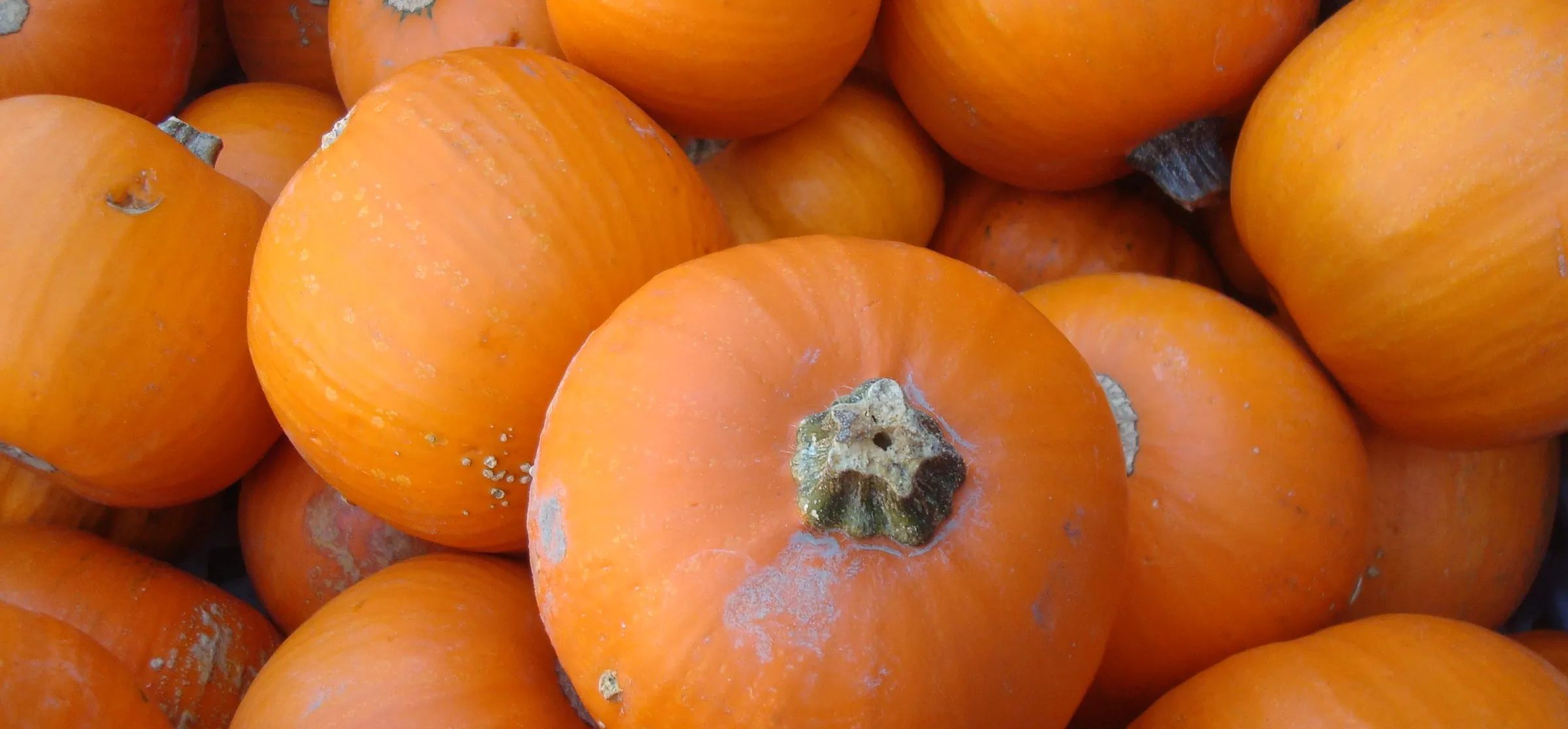
Photo: WineCountryInn (Wikivoyage) / Public domain / Wikimedia Commons
A data science case study: when the stock is bought, when shoppers actually buy, and how much a store should order when it can't know.
Americans are expected to spend a record $13.5 billion on Halloween this year, about $115 per person, according to the National Retail Federation. The money splits almost evenly three ways: costumes ($4.4 billion), decorations ($4.3 billion), and candy ($4.1 billion).
Shoppers see one night. For the businesses behind it, Halloween is a project that runs most of the year: plan, buy, make, ship, hire, sell, and clear out what's left. Most of the money is committed long before anyone knows how the season will go.
This case study uses two public retail datasets from Hugging Face to measure that gap:
- A gift wholesaler's orders show how far ahead shops buy seasonal stock.
- Walmart's daily sales show when shoppers actually buy, and we can find the Halloween products from sales alone, without product names.
- A forecasting test shows how early anyone could know how much to stock.
- A finance model turns that uncertainty into an order size.
Every step is code you can run. Use the buttons above to download the notebook or open it in Google Colab.
Setup
The standard Python data stack, plus huggingface_hub to download the data and openpyxl to read one Excel file.
pip install pandas numpy plotly huggingface_hub openpyxl
Show code · In [1]
import os
import warnings

# keep the output to results: no download progress bars or library notices
os.environ["HF_HUB_DISABLE_PROGRESS_BARS"] = "1"
warnings.filterwarnings("ignore")

import numpy as np
import pandas as pd
import plotly.express as px
import plotly.graph_objects as go
import plotly.io as pio
from huggingface_hub import hf_hub_download
from huggingface_hub.utils import logging as hf_logging

hf_logging.set_verbosity_error()

# one look for every chart: dark, transparent, and colorblind-friendly
COLORS = {"Halloween": "#fb923c", "Christmas": "#34d399", "Everything else": "#94a3b8", "Last year": "#a78bfa", "Sales pace": "#38bdf8"}
pio.templates["post"] = go.layout.Template(
    layout=dict(
        paper_bgcolor="rgba(0,0,0,0)",
        plot_bgcolor="rgba(0,0,0,0)",
        font=dict(family="Inter, system-ui, sans-serif", color="#cbd5e1", size=13),
        title=dict(font=dict(size=17, color="#f1f5f9"), x=0, xanchor="left"),
        xaxis=dict(gridcolor="rgba(148,163,184,0.15)", zerolinecolor="rgba(148,163,184,0.3)"),
        yaxis=dict(gridcolor="rgba(148,163,184,0.15)", zerolinecolor="rgba(148,163,184,0.3)"),
        colorway=list(COLORS.values()),
        margin=dict(l=10, r=10, t=60, b=10),
        legend=dict(bgcolor="rgba(0,0,0,0)"),
    )
)
pio.templates.default = "plotly_dark+post"
# show charts in JupyterLab and VS Code, and keep their data in the saved notebook
pio.renderers.default = "plotly_mimetype+notebook_connected"
1. The size of the night
The NRF has surveyed Halloween spending every year for two decades. The last six years:
| Year | Total spending | Note |
|---|---|---|
| 2021 | $10.1 billion | |
| 2022 | $10.6 billion | |
| 2023 | $12.2 billion | Record at the time |
| 2024 | $11.6 billion | A dip |
| 2025 | $13.1 billion | Record |
| 2026 | $13.5 billion | Forecast, from a survey of 7,889 adults taken September 1 to 9 |
This year's survey also found that 74% of Americans plan to celebrate, about half started shopping in September or earlier, and 79% expect tariffs to push Halloween prices up.
Show code · In [2]
# NRF annual Halloween surveys (Prosper Insights & Analytics); 2026 is a forecast
nrf = pd.DataFrame({
    "year": ["2021", "2022", "2023", "2024", "2025", "2026"],
    "billions": [10.14, 10.6, 12.2, 11.6, 13.1, 13.5],
})
nrf["kind"] = np.where(nrf["year"] == "2026", "Forecast", "Survey")

nrf_fig = px.bar(
    nrf, x="year", y="billions", color="kind", text="billions",
    color_discrete_map={"Survey": COLORS["Everything else"], "Forecast": COLORS["Halloween"]},
    title="U.S. Halloween spending keeps setting records",
    labels={"year": "", "billions": "Billions of dollars", "kind": ""},
)
nrf_fig.update_traces(texttemplate="$%{text:.1f}B", textposition="outside", hovertemplate="%{x}: $%{y:.1f} billion<extra></extra>")
nrf_fig.update_layout(yaxis_range=[0, 15.5], height=380)
nrf_fig.show()
Loading interactive chart...
2. The Halloween year
Here is the year behind one night, laid out like a project plan. The steps overlap, and the dates are a typical calendar, with real 2026 milestones where they are known. Hover over a bar for the details.
Show code · In [3]
steps = pd.DataFrame([
    ("Plan", "2025-11-01", "2026-02-28", "Review what sold and what was left over; set next year's budget and product mix"),
    ("Buy", "2026-01-15", "2026-05-31", "Trade shows and purchase orders; TransWorld's Halloween & Attractions Show ran March 26-29 in St. Louis"),
    ("Make and ship", "2026-03-15", "2026-08-31", "Factories produce and goods move to warehouses; wholesale shoppers stock up in late summer"),
    ("Hire and open", "2026-06-11", "2026-09-07", "Spirit Halloween announced 52,000 seasonal hires on June 11 and opened about 1,575 pop-up stores, most in August"),
    ("Sell", "2026-09-01", "2026-10-31", "About half of shoppers start in September or earlier, but sales pile up in the final weeks"),
    ("Clear", "2026-11-01", "2026-11-30", "Markdowns; leftovers sold off or stored; next year's plan starts"),
], columns=["step", "start", "end", "detail"])

timeline = px.timeline(
    steps, x_start="start", x_end="end", y="step", custom_data=["detail"],
    title="One night of sales, a year of work",
    color_discrete_sequence=[COLORS["Halloween"]],
)
timeline.update_traces(hovertemplate="<b>%{y}</b><br>%{customdata[0]}<extra></extra>")
timeline.update_yaxes(autorange="reversed", title="")
timeline.add_vline(x=pd.Timestamp("2026-10-31").timestamp() * 1000, line_dash="dot", line_color="#f1f5f9")
timeline.add_annotation(x="2026-10-31", y=1.06, yref="paper", text="Oct 31", showarrow=False, font=dict(color="#f1f5f9"))
timeline.update_layout(height=360, xaxis_title="")
timeline.show()
Loading interactive chart...
3. How far ahead do shops buy?
The Online Retail II dataset is two years of orders from a U.K. online gift company, December 2009 to December 2011, published by the UCI Machine Learning Repository. Many of its customers are small shops buying stock to resell, so its order dates show when retailers buy, not when shoppers do.
Show code · In [4]
path = hf_hub_download("michaelmallari/online-retail-ii", "online-retail-ii.xlsx", repo_type="dataset")
sheets = pd.read_excel(path, sheet_name=None, dtype={"Invoice": str, "StockCode": str, "Description": str})
orders = pd.concat(sheets.values(), ignore_index=True)

# keep real sales: drop returns (invoice numbers starting with C), zero prices, and negative quantities
orders = orders[(orders["Quantity"] > 0) & (orders["Price"] > 0) & ~orders["Invoice"].str.startswith("C")].copy()
orders["revenue"] = orders["Quantity"] * orders["Price"]
print(f"{len(orders):,} order lines, {orders['InvoiceDate'].min():%b %Y} to {orders['InvoiceDate'].max():%b %Y}")
print(f"{orders['Customer ID'].nunique():,} customers in {orders['Country'].nunique()} countries")
1,041,670 order lines, Dec 2009 to Dec 2011 5,878 customers in 43 countries
First, find the seasonal products by name. A catch: Halloween is a small holiday in the U.K., and this company sold only two Halloween products in two years. Christmas is its big season, so Christmas stands in here. The question is the same: how long before the holiday does the stock get bought?
Show code · In [5]
desc = orders["Description"].fillna("").str.upper()
for name, pattern in {"Christmas": "CHRISTMAS|XMAS|SANTA|REINDEER|ADVENT", "Halloween": "HALLOWEEN"}.items():
    match = desc.str.contains(pattern)
    print(f"{name}: {desc[match].nunique()} products, £{orders.loc[match, 'revenue'].sum():,.0f} in sales")

christmas = orders[desc.str.contains("CHRISTMAS|XMAS|SANTA|REINDEER|ADVENT")].copy()
# days from each order to the next Christmas
target = pd.to_datetime(christmas["InvoiceDate"].dt.year.astype(str) + "-12-25")
target = target.where(christmas["InvoiceDate"] <= target, target + pd.DateOffset(years=1))
christmas["days_before"] = (target - christmas["InvoiceDate"]).dt.days
Christmas: 231 products, £903,940 in sales Halloween: 2 products, £1,014 in sales
For every Christmas order, count the days until the next December 25, then add up the sales by month.
Show code · In [6]
lead = (
    christmas.assign(months_before=christmas["days_before"] // 30)
    .groupby("months_before")["revenue"].sum()
    .pipe(lambda s: s / s.sum())
    .loc[:6]
)
lead_fig = px.bar(
    x=lead.index, y=lead.values,
    color_discrete_sequence=[COLORS["Christmas"]],
    title="Shops order Christmas stock one to three months ahead",
    labels={"x": "Months before Christmas", "y": "Share of Christmas orders"},
)
lead_fig.update_traces(hovertemplate="%{x} to %{x}+1 months before: %{y:.0%} of orders<extra></extra>")
lead_fig.update_layout(xaxis_autorange="reversed", yaxis_tickformat=".0%", xaxis_dtick=1, height=400)
lead_fig.show()

share = lambda days: christmas.loc[christmas["days_before"] >= days, "revenue"].sum() / christmas["revenue"].sum()
print(f"Ordered at least 1 month ahead: {share(30):.0%}   2 months: {share(60):.0%}   3 months: {share(90):.0%}")
Loading interactive chart...
Ordered at least 1 month ahead: 80% 2 months: 45% 3 months: 20%
Four out of five Christmas orders came in at least a month before Christmas, and almost half came in two months or more ahead. These are small shops buying from a wholesaler that ships in days. Big chains buying straight from overseas factories have to commit earlier still, which is what the Buy and Make and ship bars on the calendar show.
4. When do shoppers buy?
The M5 dataset is five years of daily unit sales for 3,049 Walmart products in 10 stores in California, Texas, and Wisconsin, released for the M5 forecasting competition. It has one twist: product names are hidden. Every product is a code like HOBBIES_2_028, grouped into seven departments.
Show code · In [7]
calendar = pd.read_csv(hf_hub_download("denephew/M5_Forecasting", "calendar.csv", repo_type="dataset"))
sales = pd.read_csv(hf_hub_download("denephew/M5_Forecasting", "sales_train_evaluation.csv", repo_type="dataset"))

day_cols = [c for c in sales.columns if c.startswith("d_")]
dates = pd.DatetimeIndex(pd.to_datetime(calendar.set_index("d").loc[day_cols, "date"]))

# add up all 10 stores: one row per product, one column per day
items = sales.groupby(["item_id", "dept_id"])[day_cols].sum()
items.columns = dates
print(f"{len(items):,} products in {items.index.get_level_values('dept_id').nunique()} departments, {items.shape[1]:,} days ({dates[0]:%b %d, %Y} to {dates[-1]:%b %d, %Y})")
print("Halloween in the calendar:", ", ".join(calendar.loc[calendar["event_name_1"] == "Halloween", "date"]))
3,049 products in 7 departments, 1,941 days (Jan 29, 2011 to May 22, 2016) Halloween in the calendar: 2011-10-31, 2012-10-31, 2013-10-31, 2014-10-31, 2015-10-31
Finding the Halloween aisle without product names
If names are hidden, let the sales speak. A Halloween product should sell much faster in the three weeks before October 31 than in late summer, and then drop off right after. The test below flags a product if its sales in the final three weeks run at least 1.8 times its late-summer rate and at least 1.8 times its rate in the two weeks after Halloween, in at least three of the five years. Requiring it year after year keeps out products that just happened to have a good October once.
Show code · In [8]
YEARS = range(2011, 2016)
cols = items.columns

def daily_rate(year, start, end):
    """Average units per day for every product, from `start` to `end` days around Halloween."""
    halloween = pd.Timestamp(year, 10, 31)
    window = (cols >= halloween + pd.Timedelta(days=start)) & (cols <= halloween + pd.Timedelta(days=end))
    return items.loc[:, window].mean(axis=1)

# a Halloween product sells at least 1.8x faster in the 3 weeks before Oct 31
# than in late summer AND than in the 2 weeks after, in at least 3 of the 5 years
hits = pd.DataFrame({
    year: (daily_rate(year, -20, 0) > 1.8 * daily_rate(year, 1, 14) + 0.05)
    & (daily_rate(year, -20, 0) > 1.8 * daily_rate(year, -90, -50) + 0.05)
    for year in YEARS
})
is_halloween = hits.sum(axis=1) >= 3
halloween_items = items[is_halloween]
print(f"{is_halloween.sum()} of {len(items):,} products pass the test")
halloween_items.index.get_level_values("dept_id").value_counts().rename("products").to_frame()
15 of 3,049 products pass the test
| products | |
|---|---|
| dept_id | |
| HOBBIES_2 | 13 |
| FOODS_1 | 1 |
| FOODS_3 | 1 |
Only 15 of 3,049 products pass, and 13 of them sit in one department, HOBBIES_2. The test never looked at departments, so that clustering is a good sign it found something real. The whole department tells the same story: in the week before Halloween it sells almost twice what it sells in the week after.
Show code · In [9]
depts = items.groupby(level="dept_id").sum()
ratio = pd.DataFrame({
    year: depts.loc[:, (cols >= f"{year}-10-25") & (cols <= f"{year}-10-31")].mean(axis=1)
    / depts.loc[:, (cols >= f"{year}-11-01") & (cols <= f"{year}-11-07")].mean(axis=1)
    for year in YEARS
}).mean(axis=1).sort_values()

dept_fig = px.bar(
    x=ratio.values, y=ratio.index, orientation="h",
    color=np.where(ratio.index == "HOBBIES_2", "Halloween", "Everything else"),
    color_discrete_map=COLORS,
    title="One department sells almost twice as much the week before Halloween",
    labels={"x": "Sales in the week before Oct 31 vs. the week after", "y": ""},
)
dept_fig.add_vline(x=1, line_dash="dot", line_color="#f1f5f9")
dept_fig.update_traces(hovertemplate="%{y}: %{x:.2f}x<extra></extra>")
dept_fig.update_layout(showlegend=False, height=380, xaxis_ticksuffix="x")
dept_fig.show()
Loading interactive chart...
Now the shape of the season. The chart below averages the 15 products' daily sales over the five Halloweens, scaled so a normal late-summer day equals 1.
Show code · In [10]
# average each group's daily sales around Halloween across 2011-2015, scaled so late summer = 1
def profile(rows):
    curves = []
    for year in YEARS:
        halloween = pd.Timestamp(year, 10, 31)
        window = (cols >= halloween - pd.Timedelta(days=90)) & (cols <= halloween + pd.Timedelta(days=20))
        daily = rows.loc[:, window].sum(axis=0).values
        curves.append(daily / daily[:40].mean())
    return np.mean(curves, axis=0)

offsets = np.arange(-90, 21)
shape = pd.DataFrame({
    "days": np.tile(offsets, 2),
    "index": np.concatenate([profile(halloween_items), profile(items[~is_halloween])]),
    "group": np.repeat([f"The {len(halloween_items)} Halloween products", "Everything else"], len(offsets)),
})
shape_fig = px.line(
    shape, x="days", y="index", color="group",
    color_discrete_sequence=[COLORS["Halloween"], COLORS["Everything else"]],
    title="Halloween products build for weeks, then fall off a cliff on Nov 1",
    labels={"days": "Days from Halloween", "index": "Daily sales (late summer = 1)", "group": ""},
)
shape_fig.add_vline(x=0, line_dash="dot", line_color="#f1f5f9")
shape_fig.update_traces(hovertemplate="%{x} days: %{y:.1f}x<extra></extra>")
shape_fig.update_layout(height=420, legend=dict(orientation="h", y=1.02, x=0, yanchor="bottom"))
shape_fig.show()
Loading interactive chart...
Sales stay close to normal through September, climb through October, peak in the last days, and collapse on November 1. Everything else in the store barely moves. How late does the money arrive?
Show code · In [11]
# what share of the Sep 1 to Oct 31 season has sold by each day?
def season_mask(year):
    return (cols >= f"{year}-09-01") & (cols <= f"{year}-10-31")

curves = []
for year in YEARS:
    daily = halloween_items.loc[:, season_mask(year)].sum(axis=0).values
    curves.append(np.cumsum(daily) / daily.sum())
sold = np.mean(curves, axis=0)
days_left = np.arange(len(sold) - 1, -1, -1)
half_point = days_left[np.argmax(sold >= 0.5)]
print(f"Half of the season's units sell in the last {half_point} days before Halloween")
print(f"Sold by Oct 1: {sold[30]:.0%}   by Oct 15: {sold[44]:.0%}   by Oct 24: {sold[53]:.0%}")
Half of the season's units sell in the last 18 days before Halloween Sold by Oct 1: 27% by Oct 15: 55% by Oct 24: 76%
5. How early can anyone know?
Half of the Halloween season's units sell in the last 18 days. That raises the question every buyer faces: when do you know how much you will sell?
We test two simple forecasts of each product's season (September 1 to October 31), on the four seasons from 2012 to 2015:
- Last year: each product will sell what it sold last season. This is all a buyer has in the spring, when orders are placed.
- Sales pace: take this season's sales so far and scale them up by how much of last season had sold by the same day. If 20% of last season had sold by October 1 and this year has sold 400 units by October 1, forecast 2,000.
The score is the average miss per product: add up how far off each product's forecast was, in either direction, and divide by the total actually sold. 0% is perfect.
Show code · In [12]
season = pd.DataFrame({year: halloween_items.loc[:, season_mask(year)].sum(axis=1) for year in YEARS})

def wape(forecast, actual):
    """Total miss across products, as a share of what actually sold."""
    return np.abs(forecast - actual).sum() / actual.sum()

rows = []
for days_out in range(60, 0, -1):
    for year in range(2012, 2016):
        this_cut = pd.Timestamp(year, 10, 31) - pd.Timedelta(days=days_out)
        last_cut = pd.Timestamp(year - 1, 10, 31) - pd.Timedelta(days=days_out)
        so_far = halloween_items.loc[:, (cols >= f"{year}-09-01") & (cols <= this_cut)].sum(axis=1)
        last_so_far = halloween_items.loc[:, (cols >= f"{year - 1}-09-01") & (cols <= last_cut)].sum(axis=1)
        share_sold_by_now = last_so_far.sum() / season[year - 1].sum()
        rows.append({
            "days": days_out, "year": year,
            "Last year": wape(season[year - 1], season[year]),
            "Sales pace": wape(so_far / share_sold_by_now, season[year]),
        })
errors = pd.DataFrame(rows).groupby("days")[["Last year", "Sales pace"]].mean()

err_fig = px.line(
    errors.reset_index().melt(id_vars="days", var_name="method", value_name="miss"),
    x="days", y="miss", color="method", color_discrete_map=COLORS,
    title="A good forecast shows up about three weeks before Halloween: too late to reorder",
    labels={"days": "Days before Halloween", "miss": "Average miss per product", "method": "Forecast"},
)
err_fig.update_traces(hovertemplate="%{x} days out: off by %{y:.0%}<extra></extra>")
err_fig.update_layout(xaxis_autorange="reversed", yaxis_tickformat=".0%", height=420, yaxis_rangemode="tozero")
err_fig.show()

crossover = errors.index[errors["Sales pace"] < errors["Last year"]].max()
print(f"Last year's sales, used as the forecast, miss by {errors['Last year'].iloc[0]:.0%} per product")
print(f"Tracking this year's sales pace beats that only from {crossover} days out")
Loading interactive chart...
Last year's sales, used as the forecast, miss by 40% per product
Tracking this year's sales pace beats that only from 23 days out
Last year's sales miss by about 40% per product. Tracking this year's pace is worse for most of the season, because early sales are small and noisy, and it only pulls ahead about three weeks before Halloween.
That is the core problem in one chart. The orders were placed months ago, and a forecast worth trusting arrives about three weeks before the holiday, when there is no time left to make, ship, and shelve more. The buyer has to commit with a 40% miss baked in.
6. The finance: how much to order when you can't know
Operations research has a name for this: the newsvendor problem, after a newspaper seller deciding how many papers to buy before knowing how many will sell. Order too few and you lose sales. Order too many and you eat the leftovers. The answer depends on which mistake costs more:
- Cost of being short: the profit lost on each sale you miss (price minus cost).
- Cost of being over: what you lose on each leftover (cost minus what it brings on clearance after November 1).
The rule: order enough to cover demand in this share of seasons: short ÷ (short + over).
To get the uncertainty, we use the 15 Walmart products: for each product and year, how this season's sales compared with last season's. Then we try two made-up products and find the order size, as a share of last year's sales, that earns the most on average.
Show code · In [13]
# how this year's season compared with last year's, product by product
ratios = pd.concat([
    season[year] / season[year - 1] for year in range(2012, 2016)
])[pd.concat([season[year - 1] for year in range(2012, 2016)]) >= 20].values
print(f"{len(ratios)} product-years. This year as a share of last year: "
      f"10th percentile {np.percentile(ratios, 10):.0%}, median {np.median(ratios):.0%}, 90th percentile {np.percentile(ratios, 90):.0%}")

# two products, per unit: what it costs, what it sells for, what's left is worth after Nov 1
PRODUCTS = {
    "Costume: cost $10, price $30, clears at $5": (10, 30, 5),
    "Candy: cost $3, price $4, clears at $2": (3, 4, 2),
}
buy = np.linspace(0.4, 2.0, 161)  # order size as a multiple of last year's sales
curves, best = [], {}
for name, (cost, price, clearance) in PRODUCTS.items():
    profit = np.array([
        np.mean(price * np.minimum(q, ratios) + clearance * np.maximum(q - ratios, 0) - cost * q)
        for q in buy
    ])
    profit = profit / profit.max()
    best[name] = buy[profit.argmax()]
    curves.append(pd.DataFrame({"buy": buy, "profit": profit, "product": name}))
    critical = (price - cost) / (price - clearance)
    print(f"{name}: short costs ${price - cost:.2f}, over costs ${cost - clearance:.2f}, "
          f"so aim to cover demand {critical:.0%} of the time -> order {best[name]:.0%} of last year "
          f"(ordering exactly last year's amount gives up {1 - profit[np.argmin(abs(buy - 1))]:.0%} of the best profit)")

nv_fig = px.line(
    pd.concat(curves), x="buy", y="profit", color="product",
    color_discrete_sequence=[COLORS["Halloween"], COLORS["Last year"]],
    title="A fat margin justifies a bigger order. A thin one does not.",
    labels={"buy": "Order size (last year's sales = 100%)", "profit": "Expected profit (best = 1)", "product": ""},
)
for (name, q), color in zip(best.items(), [COLORS["Halloween"], COLORS["Last year"]]):
    nv_fig.add_vline(x=q, line_dash="dot", line_color=color)
nv_fig.update_traces(hovertemplate="Order %{x:.0%} of last year: %{y:.2f}<extra></extra>")
nv_fig.update_layout(xaxis_tickformat=".0%", yaxis_range=[0, 1.05], height=440,
                     legend=dict(orientation="h", y=1.02, x=0, yanchor="bottom"))
nv_fig.show()
52 product-years. This year as a share of last year: 10th percentile 77%, median 108%, 90th percentile 155% Costume: cost $10, price $30, clears at $5: short costs $20.00, over costs $5.00, so aim to cover demand 80% of the time -> order 142% of last year (ordering exactly last year's amount gives up 9% of the best profit) Candy: cost $3, price $4, clears at $2: short costs $1.00, over costs $1.00, so aim to cover demand 50% of the time -> order 106% of last year (ordering exactly last year's amount gives up 1% of the best profit)
Loading interactive chart...
Same data, same uncertainty, very different orders:
- The costume makes $20 a sale and loses only $5 on a leftover, so running out is the expensive mistake. The best order is about 142% of last year. Ordering exactly last year's amount gives up about 9% of the possible profit.
- The candy makes $1 a sale and loses $1 on a leftover. The mistakes cost the same, so the best order is near the middle of the range, about 106% of last year.
This is why the clearance price after November 1 is part of the buying decision, not an afterthought. The more a leftover is worth, the bigger the order a store can afford.
7. Takeaways
The decision comes before the data
Stock is bought months ahead. Four in five of the wholesaler's Christmas orders came in at least a month early, and big chains buying from factories commit earlier still. A useful forecast shows up about three weeks before Halloween. The job is not to forecast perfectly. It is to decide how wrong the business can afford to be.
Sales arrive late and stop at midnight
Half of the Halloween products' units sell in the last 18 days, and sales fall off a cliff on November 1. A store that is out of stock in the final week has missed the biggest part of its season, and a store with too much on November 1 is selling at clearance prices.
Order size is a finance decision
The same 40% forecast miss leads to very different orders depending on margin and clearance value. High margins and cheap leftovers justify buying well over last year. Thin margins call for buying close to the expected demand.
Ways to shorten the gap
The calendar suggests where businesses fight back: suppliers close enough to restock mid-season, pop-up stores that sign short leases, seasonal staff hired for the weeks that matter, and clearance and storage plans for what's left. Spirit Halloween does several of these: it opens about 1,575 temporary stores, hires 52,000 seasonal workers, and says it carries over very little stock, storing unsold costumes that are still in good condition for the next season.
Limits
- The Walmart data hides product names, so the 15 products are inferred from their sales. They are probably everyday products that Halloween lifts, like party supplies and treats, since short-lived seasonal products tend not to have years of history.
- Walmart's weekly prices in this data barely move around Halloween, so markdowns can't be measured here.
- The wholesaler is British and barely sells Halloween, so Christmas stands in for buying lead times.
- The costume and candy prices in Section 6 are made up to show how the math works.
Sources
- National Retail Federation, Halloween Data and Trends, 2026 survey with Prosper Insights & Analytics.
- Talk Business & Politics, NRF: 2026 Halloween spending expected to rise, September 2026, past years' totals.
- Spirit Halloween, Spirit summons 52,000 seasonal associates, June 11, 2026.
- Patch, Spirit Halloween is back in Tucson, 2026, store count.
- CNBC, Spirit Halloween lives on when the holiday ends, November 1, 2023.
- Explore St. Louis, TransWorld's Halloween & Attractions Show, March 2026.
- Chen, D. (2019). Online Retail II. UCI Machine Learning Repository, CC BY 4.0. Hugging Face mirror.
- Makridakis, S., Spiliotis, E., and Assimakopoulos, V. (2022). M5 accuracy competition: Results, findings, and conclusions. International Journal of Forecasting, 38(4). Data: Hugging Face mirror.
Comments?
React, share it, or leave a comment below.
Write your thoughts?
No comments yet. Start the conversation.
Existing comments couldn't be loaded right now. You can still post one.