Can a Language Model Pick Your Features?
Can an AI guess which data matters without ever seeing the data? A small experiment pits a language model against two standard methods on 1994 census data, with the full notebook to run yourself.
 Christopher A. Rotunno 15 min read
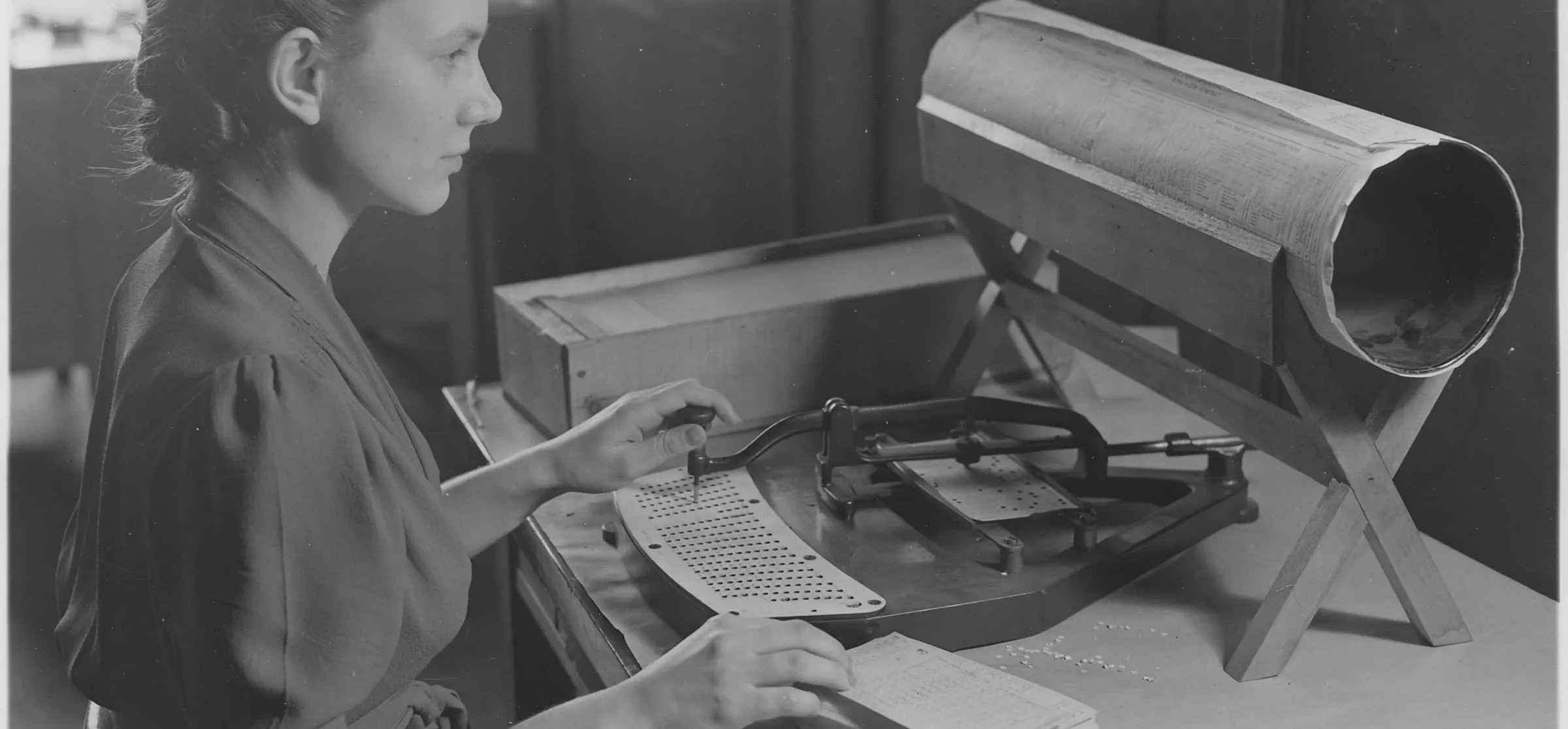
Photo: U.S. Census Bureau / Public domain / Wikimedia Commons
A small experiment: can an AI guess which data matters, without ever seeing the data?
When you build a model to predict something, you first decide which pieces of information to give it. Those pieces are called features. Picking them well matters: give the model junk and it learns noise; leave out something important and it misses the pattern.
Normally you pick features by looking at the data. This experiment tries something different. We give an AI language model only the names and short descriptions of each column, the way you would hand a new analyst a data dictionary, and ask which ones should matter for predicting income. It never sees a single number. Then we check its picks against two standard methods that do look at the data.
The idea comes from a 2024 paper, LLM-Select (Jeong, Lipton, and Ravikumar), which found that large AI models can rank features about as well as classic methods. This post tries it with a smaller, open model running on a local machine.
The short version
- The AI has good common sense. It spotted a column that is pure census bookkeeping and scored it last. One of the two data methods was fooled by it.
- But it missed the surprise in the data. Marital status turned out to be one of the strongest signals of income. The AI guessed it was weak.
- On the final test, it was only a little better than picking at random. Its ranking beat 70% of random orderings; the two data methods beat 97% and 100%.
- Verdict: an AI is a useful brainstorming partner before you have data. The data should make the final call.
Terms used below, in plain English
| Term | Meaning |
|---|---|
| Feature | One column of information about each person, like age or job |
| Model | A program that learns patterns from examples, then makes predictions |
| AUC | The score models are graded with: 0.5 is a coin flip, 1.0 is perfect |
| Ranking | A method's list of features, from most useful to least |
| Section | What happens |
|---|---|
| 1. The data | Meet 32,561 people from the 1994 U.S. Census |
| 2. A baseline model | Train a model on every feature, to get a score to beat |
| 3. Method one: a statistics test | Measure how closely each feature tracks income |
| 4. Method two: ask the trained model | Scramble each feature and see how much the model suffers |
| 5. Method three: ask the AI | Score each feature from its description alone |
| 6. Comparing the rankings | Where the three methods agree and disagree |
| 7. The real test | Build models from each method's top picks |
| 8. Takeaways | What worked, what didn't, and whether the idea is any good |
Running it yourself: every cell runs anywhere. Section 5 can call any AI model with an OpenAI-compatible API (llama.cpp, Ollama, vLLM, or a hosted service). Without one, it loads the saved scores from this post, so you get the same results.
Setup
The libraries are the standard Python data stack plus two extras: datasets to pull the data from Hugging Face, and openai, which is only used as a client for whichever language model you point it at.
pip install pandas scikit-learn plotly datasets openai scipy
The model settings come from environment variables so nothing secret lives in the notebook. The defaults point at a local llama.cpp server running MiniCPM-V 4.7 35B-A3B, an open-weights mixture-of-experts transformer. To use Mistral NeMo instead, run ollama pull mistral-nemo and set LLM_BASE_URL=http://localhost:11434/v1 and LLM_MODEL=mistral-nemo.
Show code · In [1]
import json
import os
import re
import warnings
from pathlib import Path

# keep the output to results: no download progress bars or library notices
os.environ["HF_HUB_DISABLE_PROGRESS_BARS"] = "1"
os.environ["HF_DATASETS_DISABLE_PROGRESS_BARS"] = "1"
warnings.filterwarnings("ignore")

import numpy as np
import pandas as pd
import plotly.express as px
import plotly.graph_objects as go
import plotly.io as pio
from datasets import load_dataset
from huggingface_hub.utils import logging as hf_logging
from sklearn.ensemble import HistGradientBoostingClassifier
from sklearn.feature_selection import mutual_info_classif
from sklearn.inspection import permutation_importance
from sklearn.metrics import roc_auc_score
from sklearn.model_selection import RepeatedStratifiedKFold, cross_val_score, train_test_split

hf_logging.set_verbosity_error()
RANDOM_STATE = 42

# language model settings (any OpenAI-compatible server)
LLM_BASE_URL = os.environ.get("LLM_BASE_URL", "http://127.0.0.1:8080/v1")
LLM_API_KEY = os.environ.get("LLM_API_KEY", "not-needed")
LLM_MODEL = os.environ.get("LLM_MODEL", "minicpm-v")
LLM_CACHE = Path("llm_feature_scores.json")
# reuse the saved scores so results are reproducible; set True to score again with your own model
REFRESH_LLM = os.environ.get("REFRESH_LLM") == "1"

# one look for every chart: dark, transparent, and colorblind-friendly
COLORS = {"Mutual information": "#38bdf8", "Permutation importance": "#a78bfa", "Language model": "#34d399", "Random": "#94a3b8"}
pio.templates["post"] = go.layout.Template(
    layout=dict(
        paper_bgcolor="rgba(0,0,0,0)",
        plot_bgcolor="rgba(0,0,0,0)",
        font=dict(family="Inter, system-ui, sans-serif", color="#cbd5e1", size=13),
        title=dict(font=dict(size=17, color="#f1f5f9"), x=0, xanchor="left"),
        xaxis=dict(gridcolor="rgba(148,163,184,0.15)", zerolinecolor="rgba(148,163,184,0.3)"),
        yaxis=dict(gridcolor="rgba(148,163,184,0.15)", zerolinecolor="rgba(148,163,184,0.3)"),
        colorway=list(COLORS.values()),
        margin=dict(l=10, r=10, t=60, b=10),
        legend=dict(bgcolor="rgba(0,0,0,0)"),
    )
)
pio.templates.default = "plotly_dark+post"
# show charts in JupyterLab and VS Code, and keep their data in the saved notebook
pio.renderers.default = "plotly_mimetype+notebook_connected"
1. The data
The Adult Census Income dataset comes from the 1994 U.S. Census. Each row is one person, and the question is simple: does this person earn more than $50,000 a year? It is one of the most widely used datasets in machine learning, and it hides two traps that make it a good test.
| Feature | What it means |
|---|---|
age | Age in years |
workclass | Employer type: private, self-employed, government, and so on |
fnlwgt | Census sampling weight: how many people in the population this row represents |
education | Highest level of education, as a label |
education.num | The same education level, as a number from 1 to 16 |
marital.status | Married, never married, divorced, and so on |
occupation | Broad job category |
relationship | Role in the household: husband, wife, own child, and so on |
race | Race as recorded by the census |
sex | Sex as recorded by the census |
capital.gain | Income from investment gains |
capital.loss | Losses from investments |
hours.per.week | Usual hours worked per week |
native.country | Country of origin |
Trap one: fnlwgt is not a fact about the person. It is a number the census uses to scale its sample up to the whole country, so it should tell you nothing about anyone's income. Trap two: education and education.num are the same information in two formats. A good method should ignore the first and only need one of the second.
Show code · In [2]
raw = load_dataset("scikit-learn/adult-census-income", split="train").to_pandas()

df = raw.replace("?", np.nan)
CATEGORICAL = ["workclass", "education", "marital.status", "occupation", "relationship", "race", "sex", "native.country"]
NUMERIC = ["age", "fnlwgt", "education.num", "capital.gain", "capital.loss", "hours.per.week"]
FEATURES = [f for f in raw.columns if f != "income"]

for col in CATEGORICAL:
    df[col] = df[col].fillna("Unknown").astype("category")
y = (df["income"] == ">50K").astype(int)
X = df[FEATURES]

print(f"{len(df):,} people, {len(FEATURES)} features")
print(f"{y.mean():.1%} earn more than $50K")
X.head()
32,561 people, 14 features 24.1% earn more than $50K
| age | workclass | fnlwgt | education | education.num | marital.status | occupation | relationship | race | sex | capital.gain | capital.loss | hours.per.week | native.country | |
|---|---|---|---|---|---|---|---|---|---|---|---|---|---|---|
| 0 | 90 | Unknown | 77053 | HS-grad | 9 | Widowed | Unknown | Not-in-family | White | Female | 0 | 4356 | 40 | United-States |
| 1 | 82 | Private | 132870 | HS-grad | 9 | Widowed | Exec-managerial | Not-in-family | White | Female | 0 | 4356 | 18 | United-States |
| 2 | 66 | Unknown | 186061 | Some-college | 10 | Widowed | Unknown | Unmarried | Black | Female | 0 | 4356 | 40 | United-States |
| 3 | 54 | Private | 140359 | 7th-8th | 4 | Divorced | Machine-op-inspct | Unmarried | White | Female | 0 | 3900 | 40 | United-States |
| 4 | 41 | Private | 264663 | Some-college | 10 | Separated | Prof-specialty | Own-child | White | Female | 0 | 3900 | 40 | United-States |
About one in four people (24.1%) earns more than $50K. Because of that imbalance, plain accuracy would be misleading: a model that always guessed "no" would be 76% accurate and completely useless. Instead the models are graded with AUC (short for ROC AUC). It asks: pick one high earner and one low earner at random, how often does the model rate the high earner higher? 0.5 is a coin flip; 1.0 is perfect.
Before ranking anything, two charts to get a feel for the data.
Show code · In [3]
# count ages into 2-year bins per group, so the chart carries 70 numbers instead of 32,000 rows
bins = np.arange(16, 92, 2)
age_mix = pd.concat([
    pd.DataFrame({"age": bins[:-1], "upper": bins[:-1] + 1, "share": np.histogram(df.loc[y == flag, "age"], bins=bins)[0] / (y == flag).sum(), "Income": label})
    for flag, label in [(0, "$50K or less"), (1, "More than $50K")]
])
age_fig = px.bar(
    age_mix, x="age", y="share", color="Income", barmode="overlay", opacity=0.75, custom_data=["upper"],
    color_discrete_sequence=["#94a3b8", "#34d399"],
    title="Higher earners skew older, peaking in their 40s and 50s",
    labels={"age": "Age", "share": "Share of group"},
)
age_fig.update_traces(hovertemplate="Ages %{x} to %{customdata[0]}: %{y:.1%} of the group<extra></extra>")
age_fig.update_layout(yaxis_tickformat=".0%", legend_title_text="", bargap=0.05)
age_fig.show()
Loading interactive chart...
Show code · In [4]
edu = (
    df.assign(high=y)
    .groupby("education", observed=True)
    .agg(rate=("high", "mean"), people=("high", "size"), level=("education.num", "first"))
    .sort_values("level")
    .reset_index()
)
edu_fig = px.bar(
    edu, x="education", y="rate", custom_data=["people"],
    title="The chance of earning over $50K climbs with every step of education",
    labels={"education": "", "rate": "Share earning over $50K"},
    color_discrete_sequence=["#34d399"],
)
edu_fig.update_traces(hovertemplate="%{x}<br>%{y:.0%} earn over $50K<br>%{customdata[0]:,} people<extra></extra>")
edu_fig.update_layout(yaxis_tickformat=".0%", xaxis_tickangle=-40)
edu_fig.show()
Loading interactive chart...
2. A baseline model
To grade a set of features, we need a model to test them with. We use gradient boosting, a strong, fast, standard choice for spreadsheet-style data. Think of it as hundreds of small decision trees, each one correcting the mistakes of the ones before it.
We set aside 25% of the people as a test set the model never sees while training, then grade it with AUC.
Show code · In [5]
X_train, X_test, y_train, y_test = train_test_split(X, y, test_size=0.25, stratify=y, random_state=RANDOM_STATE)


def make_model():
    return HistGradientBoostingClassifier(categorical_features="from_dtype", random_state=RANDOM_STATE)


baseline = make_model().fit(X_train, y_train)
baseline_auc = roc_auc_score(y_test, baseline.predict_proba(X_test)[:, 1])
print(f"Test ROC AUC with all {len(FEATURES)} features: {baseline_auc:.3f}")
Test ROC AUC with all 14 features: 0.922
That is the score to beat, or at least to match with fewer features. A model that is nearly as accurate with fewer inputs is usually the better model: cheaper to run, easier to explain, and less likely to break when the data changes.
3. Method one: a statistics test (mutual information)
Mutual information measures how much knowing a feature tells you about income. Zero means it tells you nothing; higher means more. It is quick and catches patterns that are not straight lines, but it judges each feature alone, so it cannot tell when two features say the same thing.
Show code · In [6]
X_codes = X_train.copy()
for col in CATEGORICAL:
    X_codes[col] = X_codes[col].cat.codes

mi = pd.Series(
    mutual_info_classif(X_codes, y_train, discrete_features=[c in CATEGORICAL for c in FEATURES], random_state=RANDOM_STATE),
    index=FEATURES,
).sort_values()

mi_fig = px.bar(
    x=mi.values, y=mi.index, orientation="h",
    title="Mutual information: relationship and marital status lead",
    labels={"x": "Mutual information with income", "y": ""},
    color_discrete_sequence=[COLORS["Mutual information"]],
)
mi_fig.update_traces(hovertemplate="%{y}: %{x:.3f}<extra></extra>")
mi_fig.show()
Loading interactive chart...
4. Method two: ask the trained model (permutation importance)
Permutation importance tests the trained model directly. For each feature, it scrambles that column, breaking its link to income, and measures how much the model's score drops. A big drop means the model relied on that feature. It is like leaving one ingredient out of a recipe to see how much the dish suffers. Each feature is scrambled ten times, and the error bars show the spread.
Unlike the statistics test, this one notices duplicates: if two features carry the same information, scrambling one barely hurts, because the model leans on the other.
Show code · In [7]
perm = permutation_importance(
    baseline, X_test, y_test, scoring="roc_auc", n_repeats=10, random_state=RANDOM_STATE, n_jobs=-1
)
pi = pd.DataFrame({"mean": perm.importances_mean, "std": perm.importances_std}, index=FEATURES).sort_values("mean")

pi_fig = px.bar(
    pi, x="mean", y=pi.index, orientation="h", error_x="std",
    title="Permutation importance: what the trained model actually relies on",
    labels={"mean": "Drop in ROC AUC when shuffled", "index": ""},
    color_discrete_sequence=[COLORS["Permutation importance"]],
)
pi_fig.update_traces(hovertemplate="%{y}: %{x:.4f}<extra></extra>")
pi_fig.update_layout(yaxis_title="")
pi_fig.show()
Loading interactive chart...
5. Method three: ask the AI
Now the experiment. We give an AI language model the same feature table a person would read, explain the task, and ask it to score each feature from 0 to 1, with a one-sentence reason.
The AI gets no data: no rows, no numbers, no statistics. Everything it knows comes from what it learned in training about how income relates to age, education, work, and so on. That is the appeal: this works before you have collected any data, and it never exposes private records to the AI.
The AI here is MiniCPM-V, an open model running locally. It is smaller than the largest models tested in the original paper, like GPT-4, so treat this as a test of what a modest model can do, not a verdict on AI in general.
AI answers vary a little each time, so we ask five times and average. The spread between runs becomes the error bar.
The scores used in this post are saved in llm_feature_scores.json and loaded by default, so your results will match. Set REFRESH_LLM = True (or the environment variable REFRESH_LLM=1) to score the features again with your own model.
Show code · In [8]
DESCRIPTIONS = {
    "age": "Age in years",
    "workclass": "Employer type: private, self-employed, government, and so on",
    "fnlwgt": "Census sampling weight: how many people in the population this row represents",
    "education": "Highest level of education, as a label",
    "education.num": "The same education level, as a number from 1 to 16",
    "marital.status": "Married, never married, divorced, and so on",
    "occupation": "Broad job category",
    "relationship": "Role in the household: husband, wife, own child, and so on",
    "race": "Race as recorded by the census",
    "sex": "Sex as recorded by the census",
    "capital.gain": "Income from investment gains",
    "capital.loss": "Losses from investments",
    "hours.per.week": "Usual hours worked per week",
    "native.country": "Country of origin",
}

PROMPT = (
    "You are helping select features for a model that predicts whether a person's annual income is above $50,000, "
    "using records from the 1994 U.S. Census.\n\n"
    "Features:\n" + "\n".join(f"- {name}: {desc}" for name, desc in DESCRIPTIONS.items()) + "\n\n"
    "For each feature, give an importance score from 0 (useless for predicting income) to 1 (extremely useful), "
    "based on your knowledge of what drives income. Score features independently; several can share a score.\n"
    'Reply with only a JSON object mapping each feature name to {"score": number, "reason": "one short sentence"}.'
)
print(PROMPT)
You are helping select features for a model that predicts whether a person's annual income is above $50,000, using records from the 1994 U.S. Census.
Features:
- age: Age in years
- workclass: Employer type: private, self-employed, government, and so on
- fnlwgt: Census sampling weight: how many people in the population this row represents
- education: Highest level of education, as a label
- education.num: The same education level, as a number from 1 to 16
- marital.status: Married, never married, divorced, and so on
- occupation: Broad job category
- relationship: Role in the household: husband, wife, own child, and so on
- race: Race as recorded by the census
- sex: Sex as recorded by the census
- capital.gain: Income from investment gains
- capital.loss: Losses from investments
- hours.per.week: Usual hours worked per week
- native.country: Country of origin
For each feature, give an importance score from 0 (useless for predicting income) to 1 (extremely useful), based on your knowledge of what drives income. Score features independently; several can share a score.
Reply with only a JSON object mapping each feature name to {"score": number, "reason": "one short sentence"}.
Show code · In [9]
N_RUNS = 5


def ask_llm(n_runs=N_RUNS):
    from openai import OpenAI

    client = OpenAI(base_url=LLM_BASE_URL, api_key=LLM_API_KEY, timeout=180)
    runs = []
    for i in range(n_runs):
        reply = client.chat.completions.create(
            model=LLM_MODEL,
            messages=[{"role": "user", "content": PROMPT}],
            temperature=0.7,
            max_tokens=1500,
        ).choices[0].message.content
        parsed = json.loads(re.search(r"\{.*\}", reply, re.S).group(0))  # tolerate text around the JSON
        runs.append({f: parsed[f] for f in FEATURES})
        print(f"run {i + 1}/{n_runs} done")
    return runs


CACHE_URL = "https://raw.githubusercontent.com/towardsuffering/rotunno.io/main/src/data/blog/en/llm-feature-selection/llm_feature_scores.json"


def load_cache():
    # opened from GitHub in Colab, the saved scores aren't next to the notebook, so fetch them
    if not LLM_CACHE.exists():
        import urllib.request

        LLM_CACHE.write_bytes(urllib.request.urlopen(CACHE_URL).read())
    return json.loads(LLM_CACHE.read_text())


if REFRESH_LLM or not (LLM_CACHE.exists() or os.environ.get("COLAB_RELEASE_TAG")):
    llm_runs = ask_llm()
    LLM_CACHE.write_text(json.dumps({"model": LLM_MODEL, "prompt": PROMPT, "runs": llm_runs}, indent=1))
    llm_model_used = LLM_MODEL
    print(f"Scored by {LLM_MODEL}; saved to {LLM_CACHE}")
else:
    cached = load_cache()
    llm_runs, llm_model_used = cached["runs"], cached["model"]
    print(f"Using saved scores from {llm_model_used} ({len(llm_runs)} runs)")
Using saved scores from minicpm-v (5 runs)
Show code · In [10]
scores = pd.DataFrame([{f: float(run[f]["score"]) for f in FEATURES} for run in llm_runs])
llm = pd.DataFrame({"mean": scores.mean(), "std": scores.std()}).sort_values("mean")
reasons = {f: llm_runs[0][f]["reason"] for f in FEATURES}

llm_fig = px.bar(
    llm, x="mean", y=llm.index, orientation="h", error_x="std",
    custom_data=[[reasons[f] for f in llm.index]],
    title=f"Language model scores ({llm_model_used}, average of {len(llm_runs)} runs)",
    labels={"mean": "Importance score (0 to 1)", "index": ""},
    color_discrete_sequence=[COLORS["Language model"]],
)
llm_fig.update_traces(hovertemplate="<b>%{y}</b>: %{x:.2f}<br>%{customdata[0]}<extra></extra>")
llm_fig.update_layout(yaxis_title="", xaxis_range=[0, 1.05])
llm_fig.show()

pd.DataFrame({"score": llm["mean"].round(2), "reason": [reasons[f] for f in llm.index]}, index=llm.index).iloc[::-1]
Loading interactive chart...
| score | reason | |
|---|---|---|
| occupation | 0.84 | The specific job category is one of the strong... |
| education.num | 0.80 | Provides the same predictive information as ed... |
| education | 0.80 | Higher education levels are strongly correlate... |
| age | 0.70 | Income generally increases with experience and... |
| capital.gain | 0.68 | Significant investment gains often indicate we... |
| hours.per.week | 0.60 | Working more hours generally leads to higher i... |
| workclass | 0.60 | Employer type often correlates with industry s... |
| sex | 0.50 | Gender pay gaps exist, making it a weak but st... |
| race | 0.44 | While systemic disparities exist, it is a sens... |
| capital.loss | 0.40 | Investment losses can indicate active investin... |
| marital.status | 0.40 | Married individuals often have higher househol... |
| relationship | 0.30 | Role in household correlates with being a prim... |
| native.country | 0.28 | Country of origin may correlate with immigrati... |
| fnlwgt | 0.06 | This is a sampling weight for population estim... |
Hover over any bar to read the AI's reasoning. Two things to check against the traps from Section 1: what did it give fnlwgt, the bookkeeping column, and did it notice that education and education.num are the same thing?
6. Comparing the rankings
Each method scores features on its own scale, so the fair comparison is by rank: 1 for the feature a method likes most, 14 for the one it likes least. The chart below follows each feature across the three methods. Flat lines mean the methods agree; steep lines mean they disagree. A few lines are drawn bolder to make them easier to follow.
Show code · In [11]
rankings = pd.DataFrame({
    "Mutual information": mi.rank(ascending=False),
    "Permutation importance": pi["mean"].rank(ascending=False),
    "Language model": llm["mean"].rank(ascending=False, method="first"),
}).loc[FEATURES]

methods = list(rankings.columns)
bump = go.Figure()
for feature, row in rankings.iterrows():
    highlight = feature in ("fnlwgt", "education", "education.num", "capital.gain")
    bump.add_trace(go.Scatter(
        x=methods, y=row.values, mode="lines+markers+text", name=feature,
        text=["", "", feature], textposition="middle right",
        line=dict(width=3 if highlight else 1.5),
        opacity=1 if highlight else 0.55,
        hovertemplate=f"<b>{feature}</b><br>%{{x}}: rank %{{y:.0f}}<extra></extra>",
    ))
bump.update_layout(
    title="How each feature ranks under each method (1 = most important)",
    yaxis=dict(autorange="reversed", title="Rank", dtick=1),
    xaxis=dict(title=""), showlegend=False, height=560, margin=dict(r=120),
)
bump.show()
Loading interactive chart...
Show code · In [12]
corr = rankings.corr(method="spearman")
corr_fig = px.imshow(
    corr, text_auto=".2f", zmin=-1, zmax=1, color_continuous_scale="Tealgrn",
    title="Rank agreement between methods (Spearman correlation)",
)
corr_fig.update_layout(coloraxis_showscale=False, height=420)
corr_fig.show()
Loading interactive chart...
The heatmap boils the chart above down to one number per pair of methods, a rank correlation: 1 means two methods put the features in the same order, 0 means no relationship. The two data methods agree strongly (0.80). The AI agrees only weakly with either one (0.27 and 0.33).
7. The real test: build models from each method's top picks
Agreement is nice, but what matters is whether a ranking builds good models. For each method, we train a model on its top 1 feature, then its top 2, and so on up to all 14, grading each one. Every grade is an average of ten tries: the training data is split into five parts, each part takes a turn as the test, and the whole thing is done twice. That way one lucky split cannot decide the result.
To see what luck alone can do, we also shuffle the features into 30 random orders and run the same test on each. The shaded band in the chart covers the middle 80% of them. A line inside the band did no better than luck; a line above it did.
A good ranking climbs fast: it gets close to the full model's score with just a handful of features.
Show code · In [13]
# grade every model with 5-fold cross-validation, repeated twice, so one lucky split can't decide the result
cv = RepeatedStratifiedKFold(n_splits=5, n_repeats=2, random_state=RANDOM_STATE)


def auc_with(features):
    return cross_val_score(make_model(), X_train[features], y_train, cv=cv, scoring="roc_auc", n_jobs=-1).mean()


orders = {method: list(rankings[method].sort_values().index) for method in methods}
ks = range(1, len(FEATURES) + 1)
curve_df = pd.DataFrame({method: [auc_with(order[:k]) for k in ks] for method, order in orders.items()}, index=list(ks))

# 30 random orders show how much luck alone can do
N_RANDOM = 30
rng = np.random.default_rng(RANDOM_STATE)
random_orders = [list(rng.permutation(FEATURES)) for _ in range(N_RANDOM)]
random_curves = np.array([[auc_with(order[:k]) for k in ks] for order in random_orders])
low, mid, high = np.percentile(random_curves, [10, 50, 90], axis=0)
full_auc = curve_df.iloc[-1, 0]

curve_fig = go.Figure()
curve_fig.add_trace(go.Scatter(
    x=list(ks) + list(ks)[::-1], y=list(high) + list(low)[::-1], fill="toself",
    fillcolor="rgba(148,163,184,0.18)", line=dict(width=0), hoverinfo="skip",
    name=f"Random: middle 80% of {N_RANDOM} orders",
))
curve_fig.add_trace(go.Scatter(
    x=list(ks), y=mid, mode="lines", name="Random: median",
    line=dict(color=COLORS["Random"], width=2, dash="dot"),
    hovertemplate="Random median<br>top %{x} features: AUC %{y:.3f}<extra></extra>",
))
for method in methods:
    curve_fig.add_trace(go.Scatter(
        x=curve_df.index, y=curve_df[method], mode="lines+markers", name=method,
        line=dict(color=COLORS[method], width=3 if method == "Language model" else 2),
        hovertemplate=f"{method}<br>top %{{x}} features: AUC %{{y:.3f}}<extra></extra>",
    ))
curve_fig.add_hline(y=full_auc, line_dash="dash", line_color="rgba(148,163,184,0.5)", annotation_text="all features")
curve_fig.update_layout(
    title="Model accuracy using only each method's top k features",
    xaxis=dict(title="Number of features used (k)", dtick=1),
    yaxis=dict(title="Cross-validated ROC AUC"),
    legend=dict(orientation="h", y=-0.2), height=520,
)
curve_fig.show()
Loading interactive chart...
Show code · In [14]
# two ways to score a whole curve: how few features reach near-full accuracy, and the average AUC across every k
target = full_auc - 0.01


def needed(curve):
    return int(np.argmax(np.asarray(curve) >= target)) + 1


random_needed = np.array([needed(c) for c in random_curves])
random_avg = random_curves.mean(axis=1)

scoreboard = pd.DataFrame({
    "Features needed": {m: needed(curve_df[m]) for m in methods},
    "Average AUC (k = 1 to 14)": curve_df[methods].mean().round(3),
    "Random orders it beats": {m: f"{(random_avg < curve_df[m].mean()).mean():.0%}" for m in methods},
})
scoreboard.loc[f"Random (median of {N_RANDOM})"] = [int(np.median(random_needed)), round(float(np.median(random_avg)), 3), ""]
print(f"Full model AUC: {full_auc:.3f}. 'Features needed' = fewest top features within 0.01 of it.")
print(f"Random orders needed anywhere from {random_needed.min()} to {random_needed.max()} features.")
scoreboard
Full model AUC: 0.928. 'Features needed' = fewest top features within 0.01 of it. Random orders needed anywhere from 7 to 14 features.
| Features needed | Average AUC (k = 1 to 14) | Random orders it beats | |
|---|---|---|---|
| Mutual information | 8 | 0.893 | 100% |
| Permutation importance | 7 | 0.891 | 97% |
| Language model | 10 | 0.864 | 70% |
| Random (median of 30) | 11 | 0.851 |
8. Takeaways
The AI scores come from the saved run (MiniCPM-V, five runs averaged). A different AI model may tell a different story, and that is worth trying.
What the AI got right: common sense
fnlwgt is census bookkeeping, not a fact about anyone. The AI scored it 0.06, last of all 14, explaining that it is "a sampling weight for population estimation, not a predictor of individual income." The trained model also put it near the bottom (13th), but only after seeing the data. The statistics test was fooled and ranked it 10th, ahead of four real features. The AI got it right from the description alone.
What it got wrong: the surprise in the data
Both data methods found that relationship and marital.status are among the strongest signals of income. The AI ranked them 12th and 10th. Its own reasoning shows it half knew why, noting that "married individuals often have higher household incomes or dual incomes," but it called that "a weak proxy." The data disagrees. A likely reason: in 1994, being married, and especially being listed as a husband, went along with being older, male, and in a two-income home, all of which track income.
It also wasted a pick. It wrote that education.num "provides the same predictive information as education," then gave both the same 0.80 score anyway, so its second and third picks were the same information. That is the flat stretch in its curve from two features to three.
The scoreboard
Two ways to score each ranking: how few of its top features it takes to get within 0.01 of the full model (AUC 0.928), and its average score across all 14 steps of the curve, which rewards climbing fast. The last column compares that average with the 30 random orders.
| Method | Features needed | Average score | Beats this share of random orders |
|---|---|---|---|
| Method two: permutation importance | 7 | 0.891 | 97% |
| Method one: mutual information | 8 | 0.893 | 100% |
| Method three: the AI | 10 | 0.864 | 70% |
| Random order (median of 30) | 11 | 0.851 |
The two data methods sit at the top of what random orders can do. The AI sits inside the random band the whole way: ahead of the typical random order with its first two picks, behind it through the middle, and level at the end. Random orders needed anywhere from 7 to 14 features, so its 10 is nothing special. The honest summary: this AI picked features a little better than chance, while the data methods did clearly better.
So, is the idea any good?
Yes, as a first draft. Not as the final judge.
- Use an AI before you have data: to brainstorm what to collect, and to flag columns that are obviously artifacts of how the data was gathered, like sampling weights, IDs, or timestamps.
- Use the data to decide: permutation importance plus a top-k test like Section 7 is simple and reliable.
- Bigger models may do better. The original paper found the largest models were competitive with data-driven methods. Whether a stronger model would have caught the marriage effect is the obvious next experiment.
Caveats
- This dataset is famous. The AI may have seen it during training, so it could be remembering rather than reasoning. If so, it did not help much.
- One dataset, one AI model, one prompt. A different combination could rank things differently. Treat this as one honest data point, not a final answer.
- Sensitive features need human judgment. Whether
raceorsexbelong in an income model is an ethical and legal question, not a statistical one.
Try it yourself
- Set
REFRESH_LLM = True, pointLLM_MODELandLLM_BASE_URLat a different model, and see whether its ranking changes. - Rewrite the prompt to warn about duplicate features and check whether
education.numdrops. - Point the notebook at another Hugging Face dataset by replacing the dataset name and the
DESCRIPTIONStable.
Comments?
React, share it, or leave a comment below.
Write your thoughts?
No comments yet. Start the conversation.
Existing comments couldn't be loaded right now. You can still post one.