R in Action: Analyzing the Iris Dataset
A hands-on walkthrough of exploratory data analysis using R's built-in Iris dataset — aggregate functions, median comparisons, and what the numbers actually tell us about species differentiation.
 Christopher A. Rotunno 3 min read

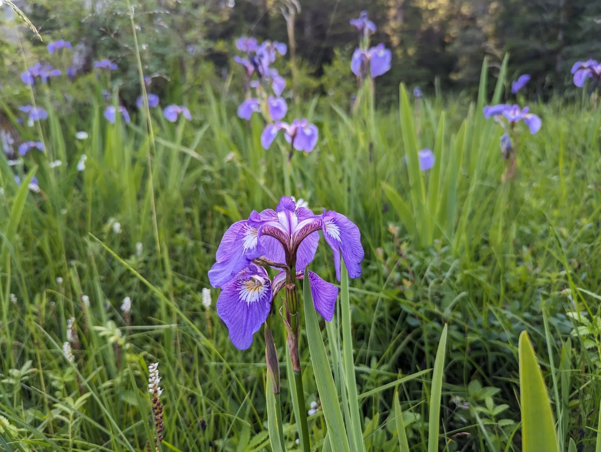
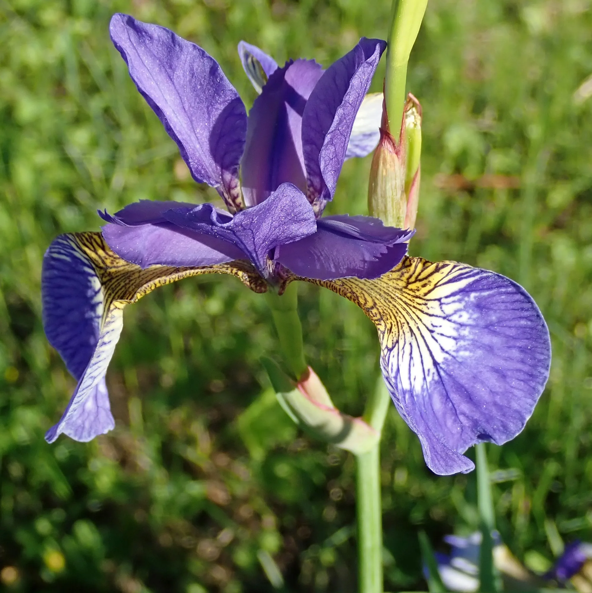
Photo: Ermell / CC BY-SA 4.0 / Wikimedia Commons
The Iris dataset is one of the most used teaching datasets in data science — and for good reason. It’s small enough to fully understand, structured enough to apply real techniques, and rich enough to surface genuine patterns. If you’ve never touched R before, it’s the right place to start. If you have, it’s a reliable benchmark for testing new methods.
This post walks through a practical EDA (Exploratory Data Analysis) using R’s built-in iris dataset, with a focus on the aggregate() function and what median sepal lengths actually reveal about the three Iris species.
The Dataset
The Iris dataset contains 150 observations across three species:
- Iris setosa
- Iris versicolor
- Iris virginica
Each observation has four measurements (in centimeters):
- Sepal length
- Sepal width
- Petal length
- Petal width

Load it in R with:
data(iris)
head(iris)
Sepal.Length Sepal.Width Petal.Length Petal.Width Species
1 5.1 3.5 1.4 0.2 setosa
2 4.9 3.0 1.4 0.2 setosa
3 4.7 3.2 1.3 0.2 setosa
4 4.6 3.1 1.5 0.2 setosa
5 5.0 3.6 1.4 0.2 setosa
6 5.4 3.9 1.7 0.4 setosaBasic Summary Statistics
Start with the basics:
summary(iris)This gives you min, max, mean, median, and quartiles for each numeric column, plus counts for the Species factor. Already useful, but not broken down by species — which is where things get interesting.
Using aggregate() for Group-Level Analysis
The aggregate() function lets you apply any function across subgroups. Syntax:
aggregate(formula, data, FUN)Mean sepal length by species:
aggregate(Sepal.Length ~ Species, data = iris, FUN = mean) Species Sepal.Length
1 setosa 5.006
2 versicolor 5.936
3 virginica 6.588Median sepal length by species:
aggregate(Sepal.Length ~ Species, data = iris, FUN = median) Species Sepal.Length
1 setosa 5.0
2 versicolor 5.9
3 virginica 6.5The mean and median are close in all three cases — which tells you the distributions are roughly symmetric, without major outliers dragging the mean away from the center.
What the Numbers Actually Say
Median sepal lengths:
- Setosa: 5.0 cm — noticeably shorter
- Versicolor: 5.9 cm — intermediate
- Virginica: 6.5 cm — consistently the largest
The gap between Setosa and Virginica is 1.5 cm — significant enough that sepal length alone has meaningful predictive power for classification. But the gap between Versicolor and Virginica is only 0.6 cm, which means sepal length alone won’t reliably separate those two.
This is why multivariate analysis matters. Let’s add petal length:
aggregate(Petal.Length ~ Species, data = iris, FUN = median) Species Petal.Length
1 setosa 1.50
2 versicolor 4.35
3 virginica 5.55Now the picture changes completely. Setosa’s median petal length is 1.5 cm. Virginica’s is 5.55 cm. That’s a 4x difference — and Setosa is trivially separable from the other two on petal length alone.
Visualizing the Distributions
Numbers are useful, but distributions tell the story better:
# Boxplot: Sepal length by species
boxplot(Sepal.Length ~ Species,
        data = iris,
        main = "Sepal Length by Species",
        xlab = "Species",
        ylab = "Sepal Length (cm)",
        col = c("#a8d8ea", "#aa96da", "#fcbad3"))
The boxplots make visible what the medians summarize: Setosa is clearly separated, while Versicolor and Virginica overlap in sepal length.
For petal length:
boxplot(Petal.Length ~ Species,
        data = iris,
        main = "Petal Length by Species",
        xlab = "Species",
        ylab = "Petal Length (cm)",
        col = c("#a8d8ea", "#aa96da", "#fcbad3"))
Here the separation is dramatic. Setosa is a tight cluster near the bottom. Versicolor and Virginica are shifted significantly upward, with limited overlap.
Adding Multiple Variables to aggregate()
You can aggregate multiple columns at once using cbind():
aggregate(cbind(Sepal.Length, Sepal.Width, Petal.Length, Petal.Width) ~ Species,
          data = iris,
          FUN = median)
Species Sepal.Length Sepal.Width Petal.Length Petal.Width
1 setosa 5.0 3.4 1.50 0.2
2 versicolor 5.9 2.8 4.35 1.3
3 virginica 6.5 3.0 5.55 2.0This single table gives you the full multivariate picture. Setosa’s petal dimensions are dramatically smaller across the board. The width measurements add texture: Setosa has the widest sepals despite being smallest overall — an interesting morphological quirk.
Key Takeaways
aggregate()is a workhorse. For grouped summaries in base R, it’s faster to write thandplyr::group_by() %>% summarize()for quick exploration — though both are valid.Median vs. mean matters when distributions aren’t symmetric. For Iris, they’re close — which is reassuring. In messy real-world data, they often diverge, and the divergence tells you something.
Single-variable analysis hides multi-variable patterns. Sepal length alone can’t reliably separate Versicolor from Virginica. Petal length changes the picture significantly.
Small datasets are still real datasets. Every EDA principle that applies here — check distributions, compare groups, look at multiple variables, visualize before modeling — applies at 150 rows and at 150 million.
What to Try Next
Once you’re comfortable with aggregate():
- Try
tapply()for applying functions to ragged arrays - Use
cor()to look at correlations between the four measurements by species - Build a simple linear discriminant analysis (LDA) with
MASS::lda()to see how well you can classify species from these four features
The Iris dataset gets more interesting the more deeply you dig into it. That’s why it’s been a teaching standard for 70 years.
Comments?
React, share it, or leave a comment below.
Write your thoughts?
No comments yet. Start the conversation.
Existing comments couldn't be loaded right now. You can still post one.